quantum hall equations
force balance
E = Vh/width = vdrift x B
vdrift = Vh/(B width)
current
i = charge-density width vdrift
vdrift = i/(charge-density width)
equate
Vh/(B width) = i/(charge-density width)
Rh = B/charge-density (in extended states)
= flux in area A/(# of electron charges in orbit of area A)
--------------------------------------------------------------------------------------------------------
The quantum
hall device is interesting both from a physics and engineering viewpoint.
Very high magnetic fields, low temperatures, and a very thin geometry cause
electrons orbiting around many tiny quantized regions of flux to become
sychronized, allowing the ratio of planck's constant to the electron's
charge (squared) to be very accurately measured. It's the world's most
accurate and stable resistor, and a classic case of how engineers and physicists
view the same device and see something different.
This essay at 35 pages is pretty comprehensive. It covers both the physics (at the semiclassical level) and engineering/circuit aspects of quantum hall, which is almost never done. On the physics side I have gathered up best physics diagrams I could locate, and on the engineering side have brought to bear my own expertise as an electrical engineer and circuit designer. I also have put numbers in all the quantum hall physics equations.
Introduction -- (conventional) hall device
Consider a
rectangular strip of semi-conducting material with current flowing in it.
Along the strip in the direction of the current flow there is voltage,
dividing this voltage by the current gives us the standard (ohms law) resistance
of the material. If you measure the voltage between the edges of the strip,
typically you would get zero, but surprisingly when a magnetic field is
turned on pointed through the wide part of the strip a (small) voltage
appears between the edges that is proportional to the magnetic field. This
side voltage is known as the hall effect voltage, after Edwin Hall who
discovered the effect in 1879, and dividing the hall voltage (Vh) by the
current (I) gives the hall resistance (Rh = Vh/I)
TheoryIntroduction -- quantum hall
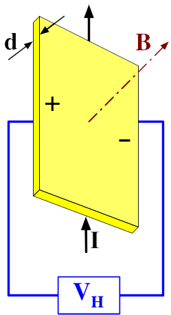
An electron moving in a magnetic field feels a sideways push, technically the electron feels a force (v cross B) that is is perpendicular both to the direction of motion and the magnetic field. As the electrons are pushed toward the side of the conductor a counterbalancing sideways electric field builds up [E = vdrift x B)]. Since vdrift is proportional to the current (I) and (Vh = E/width), in a conventional hall device the hall voltage (Vh) is proportional to the magnetic field (B) and the (longitudinal) current (I) x some dimensions of the device.
Red curve can be considered a plot of
Vhall vs B, where I = const
In a hydrogen atom an electron moves around the nucleus (proton) such that one wavelength of the electron just fits in the orbit. Something similar happens to electrons moving across a strong magnetic field. The magnetic field exerts a quadrature (right angle) force on a moving electron that causes it whirl in tight circles, called cyclotron orbits, with one (or more) wavelength just fitting in the orbit. The magnetic force on the electron is not as strong as the electromagnetic attraction between the electron and proton, so cyclotron orbits are larger, typically about 100 times larger with the cyclotron radius (@ 12.5 tesla, a strong magnetic field) at 7.5 x 10^-9 m vs hydrogen atom (ground state) electron orbit radius of 5.3 x 10^-11 m.
It turns out that in certain semiconductors with thin conducting layers at cryogenic temperatures and strong magnetic fields all the moving electrons in the device over certain ranges of B will drop into synchronized cyclotron orbits. This results in the quantum nature of the electron becoming measurable at the macro level. Not only is this very interesting in terms of the physics since it provides the physicist with an accurate way to measure fundamental electromagnetic parameters, it also provides the electrical engineer with a valuable resistance standard.
The resistance of the quantum hall device depends only on planck's constant and the electron charge (Rh = h/e^2). It turns out that this quantum hall resistance is robust, reproducible, accurate, and stable and can be very accurately measured (a part in a billion). It's the world's best resistor and since 1990 has the international resistance standard.
Fine structure constant
There's more
--- In the SI system of units the value of some terms, like c and e0, are
defined to be exact, so the hall resistance (h/e^2) scaled by exact
SI constants turns out to be the inverse of the fine structure constant
(e^2/(2 e0 hc)! The quantum hall device provides a totally independent
way to measure the dimensionless fine structure constant, which is the
electromagnetic coupling constant in QED (quantum electrodynamics).
Cracking the orbit nut?
After I had
worked out (& written up) what I though was a neat picture of quantum
hall cyclotron orbits, I found a problem. The number of electron wavelengths
around each flux quantum came out to be two, but textbooks say the
number of electron wavelengths around a cyclotron orbit must be odd
to satisfy the Pauli exclusion principle. Whoops! I was ready to throw
in the towel, when a potential solution occurred to me.
Idea -- 50/50 split of two types of orbits?
The idea is
that there are two different size orbits, each with an odd number of wavelengths,
and each corresponding to a different lobe on the energy state diagrams.
The formula for electron velocity is
v = (1/m*) sqrt{n hbar eB}
where n = 1,3,5 where n is number
of wavelengths
In the extended, current carrying, region suppose (exactly) half the electrons are encircling an (h/2e) flux quantum (with n = 1 wavelength) and the other half are encircling a three times larger area flux quantum (3h/2e) (with n = 3 wavelengths). Notice the orbit frequency, which is a measurable parameter, is the same for both orbits because in the sqrt{3}longer orbit the electrons travel sqrt{3} faster. The faster speed of electrons in the larger orbit also reduces their wavelength allowing three wavelengths to fit into the orbit.
The electrons encircling the larger flux are moving sqrt{3} faster, so they have three times the kinetic energy. Hence the one wavelength orbit represents the lowest energy lobe, and the three wavelength orbit represents the next higher energy lobe, on the energy state density diagrams the physicists draw. They draw them the same size indicating that they (probably) have the same number of states (each orbit is a state, I think). So a 50/50 split may not be so unreasonable.
Why this 50/50 split is so interesting is that its (spacial) average properties match what I calculate below. When I assumed all the orbits were the same, I found the nth plateau had n electrons encircling (h/e) flux quanta. In the two orbit picture the result is n electrons encircling the smaller (h/2e) flux quanta and n electrons encircling the 3x larger (3h/2e) flux quanta. With half of the electrons in each type of orbit we have on average two electrons in each area of (2h/e) = [(h/2e) + (3h/2e)] flux. This is an average charge density of one electron per (h/e) area of flux, exactly what I had earlier found when I assumed all the orbits were the same!
For example, dropping from the top plateau (Rh = 25.9k) to the 2nd plateau (Rh = 12.9k) occurs when B drops in half. Since [Rh = B/charge-density (in extended states)], then the charge-density (in extended states) must remain unchanged. With B halved the areas enclosed by the quantum h/2e and 3h/2e orbits double. With constant charge density that must mean that on the 2nd plateau there is now two electrons orbiting the h/2e and 3h/2e quantum fluxes. In other words going down the plateau means the # of electrons per unit area stays the same while the areas of the two quantum fluxes (still with 50/50 split) increase. Thus the number of electrons in orbit around both the h/2e and 3h/2e quantum fluxes goes up in an integer fashion (n = 1,2,3, etc) as B drops, and since the velocity is unchanged the orbit frequency drops linearly with B.
Electron orbit picture summary
Caveat -- The orbit picture below assumes that all orbits are the same, but I now think it likely that a quantum hall device has half its (extended) electrons in small orbits and half in larger orbits, representing the lowest and next lowest energy lobes of the energy state diagrams. If this is correct, then the orbit picture painted below is somewhat misleading because it represents a spacial average of these two different orbits. See 'Cracking the orbit nut' above.In this essay I derive the following semiclassical picture of cyclotron orbits of the quantum hall. I have tried to figure out (using semiclassical equations) two quantum hall issues I never see discussed: What is the orbit difference between the various plateaus, and if three or more electrons are in orbit, how are they distributed radially? My answers are the top plateau has one electron and the count increases by one for each lower plateau, and all the electrons share (somehow) the same radial space.
The conducting regions of a quantum hall device are completely full of electrons in cyclotron orbits orbiting (sort of) a double quantum flux (h/e) at a speed such that two wavelengths fit in the orbit. This is true on all the Rh plateaus of the device. The only difference between plateaus is the number of electrons in each orbit: one electron at the top plateau (Rh=25.8k), two electrons in the next plateau (Rh =12.9k), three electrons in the next plateau (Rh = 8.6k), etc. Any extra electron needed come from nearby, partially filled, localized, cyclotron orbits, where the electrons are trapped and do not contribute to the external current.
The precision of Rh on the plateaus is direct consequence of the stability of the (h/e) flux quantum ratioed to the electron charge (in the area of the flux quantum).
Rh = (h/e) quantum flux/electron charge (encircling quantum flux)
= (h/e)/ie
= h/ie^2
where i = 1,2,3,4, etc (electrons encircling (h/e) flux quantum)
For i = 1
Rh = h/e^2
= 6.6262 x 10^-34/(1.6022 x 10^-19)^2
= 25,812.8 ohm
von Klitzing's constant
The flatness of the Rh plateaus depends on the fact that the orbits smoothly (automatically) expand and contract in area as B changes, holding the encircled flux constant at the quantum value (h/e), but allowing the charge density to change as B changes.
In other words on a plateau as B increases, say 10%, the electron orbits tighten reducing the enclosed area by 10%. 10% more orbits then fit per unit area, so charge density is 10% higher. With charge density increases linearly with B, a plot of [Rh = B/charge-density (in extended states)] vs B is flat.The sequence of plateaus at all submultiple values of the von Klitzing constant (25.8k) is a direct consequence of integer increase in the electrons in the larger area orbits at lower B that holds the charge density of the conducting regions constant (at the center of the plateaus). The double flux quantum (h/e) and two wavelengths in the orbit are a direct consequence of the top plateau [flux/charge] ratio calculating to be 25.8k, von Klitzing's constant and the measured value.
How specifically more than two electrons can fit in the same radial orbit space I was unable to determine. The cyclotron orbits appear to be quite different from Bohr atomic orbits. In a Bohr atom electrons #3 to #8 orbit much further out than do electrons #1 and #2. As best as I can tell all the cyclotron electrons appear to be in the same orbit (same radial space). The explanation for how this is possible may be that electrons in this superconducting environment like to pair up and form quasi-particles that in (some sense) act like bosons rather than fermions. This sound like a recipe to violate the exclusion principle, which ordinarily limits the number of electrons in a physical orbit space to two electrons (with opposite spins).
Challenges
It took me
a long time to understand the quantum hall effect and device. This is mostly
because the physics writing on the subject is so opaque. Physicists live
in their own little world and don't seem to know how to be able to draw
clear pictures or explain fully what is going on. I know now it's possible,
because after about a month's effort I did it. Here were some of the challenges:
* Every physicist just says the longitudinal resistively is zero. Not one of the physics papers/lectures I found bothered to mention that there is a huge longitudinal resistance in a quantum hall device. Do they even know?
* The quantum hall resistance is more than a laboratory curiosity because it works well over a wide range of magnetic field strength and semiconductor charge density. I was unable to find in any physics papers/lectures a clear semi-classical explanation for why this is true. But on my own I eventually figured one out.
* You can bias a quantum hall device (by changing the magnetic field) to produce difference resistances. I figured out a semi-classical picture showing how the various hall resistance can be calculated from variations in the electron orbits (with a further complication that the orbits are apparently not all the same.)
* How do you measure hall resistance to a part in a billion? Don't ask a physicist, they don't have clue.
* When circuit guys got their hands on quantum hall, they showed how to convert it into a high quality two terminal device. To really understand this I worked up a circuit (with values) showing how external wiring resistance gets canceled out.
To help understand the quantum hall physics I also put numbers in all the equations. I even showed how (with a small stretch) quantum hall cyclotron orbits can be fit into the electron size table (in Electron essay).
Quantum hall effect -- von Klitzing constant
Starting in
the 1980's solid state physics provided a new and wholly different way
to measure the fine structure constant using the quantum Hall effect. The
hall voltage is arises directly from the coupling/interaction of a magnetic
field with moving electrons (& holes too!) in a semiconductor.
The hall voltage in a semiconductor is a small (uv to mv) voltage that develops between the sides of a conductor placed in a magnetic field. A magnetic field oriented across a conductor exerts a force [q x (vel cross B)] on the moving charges in the conductor that is perpendicular to their velocity. Essentially the magnetic field pushes the moving charges sideways a little causing a weak opposing voltage (hall voltage) to develop between the sides of the conductor. This side voltage is easily measured by putting electrodes on the sides.
The hall voltage (i B/J e d) is known from basic physics to be directly proportional to an external magnetic field (B), and there is no offset. This is unlike, say, determining planck's constant (h) from the photoelectric effect where the material introduces an offset in the straight line plot of energy vs frequency. A plot of hall voltage vs B is a straight line that goes through the origin, however, the slope of the line also depends proportionally on the bias current (i) and is inversely proportional to the density of mobile charges (J), charge e, and the thickness of the semiconductor (d).
Curiously, at low temperatures, at high magnetic fields, and in a specially built field effect transistor type hall device that has a very thin layer of free electrons under the gate (referred to as an 'electron gas'), the hall voltage is found to be quantized. A plot of hall resistance, which is hall voltage divided by current (i), shows steps of varying height as current and/or magnetic field are changed (see below). The plateau resistances are all an integer submultiple of a fixed reference value, now known as the von Klitzing constant (about 25.8 kohm). For example, the hall resistance plot might show resistance plateaus at 12.9k = 25.8k/2, 8.6k = 25.8k/3, 6.45k = 25.8k/4, etc. This integer relationship has been found to hold to one part in a billion!
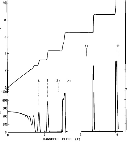
(top) hall resistance (kohm) & (bot) longitudinal
resistance vs B (tesla) (von Klitzing's 1985 Nobel lecture)
. 
(from David R Leadley quantum hall site)
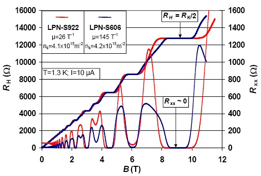
(from French Metrology Laboratoire)
The formula von Klitzing gives in his Nobel lecture is below. He derives it starting with (flux quantization) = h/e and applies this to a ring getting energy from a change of one de Broglie wavelength. He says "in this picture the main reason for the hall quantization is the flux quantization (h/e) and the quantization of charge into elementary charges (e)."
hall resistance = B/(N filled energy levels) e = h/n e^2
where
n = 1,2,3, etc
The formula for the von Klitzing constant (h/e^2) of the quantum hall effect is very simple. Notice it is just the inverse of alpha (e^2/(2 e0 hc) scaled by a (2 e0 c), but both e0 and c are vacuum parameters and are defined with no uncertainty in SI units, i.e. they are exact constants. Hence measuring the Hall voltage plateau and dividing by current (i) to get the von Klitzing constant (ohms) directly gives a value for alpha. While the electron magnetic moment yields a more accurate value for alpha, the von Klitzing constant measurement is important because it provides a significant independent confirmation of the electron magnetic moment value.
In my essay on Electrons I show alpha can be written as (e^2 Z/2h), which is the impedance of free space (Z) scaled by (e^2/2h). Since the von Klitzing constant is (h/e^2), we can write
alpha = e^2 Z/2h
=(1/2) Z /(h/e^2)
or
alpha = (1/2) impedance of free space (ohms)/von Klitzing constant (ohms)
= (1/2) 376.73031 ohm/25,812.807 ohm
= 1/137.036
dimensionless
In other words the von Klitzing constant (in ohms) comes out to be about 68.5 times (137.036/2) larger than the impedance of free space (in ohms). Klaus von Klitzing won the 1985 Nobel prize for physics for the discovery of the quantum Hall effect. Here's the link to his nobel lecture on the quantum hall effect.
http://nobelprize.virtual.museum/nobel_prizes/physics/laureates/1985/klitzing-lecture.pdf
Quantum hall effect in detail
I have long
been familiar with the Hall effect in semiconductors. I learned it in engineering
school and worked for years with current sensors that worked on the hall
principle. However, I had never learned anything about the quantum hall
effect. So before I wrote the section above, I read up using the web and
Wikipedia, and when I saw tha von Klitzing had won the 1985 Noble
prize for this work, I dug out his Nobel lecture and skimmed though it,
finding it pretty opaque.
I was unhappy that I had no real understanding of how/why the hall voltage was quantized. I had not a clue as to how the crude looking quantization in the figure above (from von Klitzing's lecture) could possibly be used to measure von Klitzing's constant, or alpha, accurately, supposedly to a part in 10 million or better! I looked through a bunch of books on quantum physics in a technical bookstore and found nothing on the quantum hall effect except the figure above. (Is it the best available?, nope) Then just thinking about it in bed a few things (seemed to) fall into place...
* Maybe the magnetic field is so strong that the drifting electrons are coiling in circles around the magnetic field lines? Yup
* Are the electrons moving something like in the Bohr atoms, in tiny circles (or spirals) quantized by the de Broglie wavelength? Sort of
Quantum hall resistance standard
The quantum
hall device is a widely used high precision resistance lab standard in
national standards labs. Resistive uncertainties are down in the 10 to
100 uhom range resulting in a (12.9k nom = (1/2) 25.8k von Klitzing constant)
resistive standard with relative uncertainties of 10^-8 to 10^-9.
Initially I didn't see how a hall device could deliver high accuracy. A (standard) hall sensor is a four terminal device with the output voltage on one set of terminals and bias current (& uncontrolled resistance) on the other. How do you use this in a bridge as a resistance standard? But it turns out that a quantum hall device is different animal. For one thing it's in a cryogenic environment where isolated currents can be servoed and ratioed very accurately using DC transformer techniques. For another the quantum hall device contains a 2Dgas that is inherently symmetrical. It's current terminals and voltage terminals have the same basic characteristics.
The standard geometry of a quantum hall device is current terminals on the ends (current typ 50 ua) and three sets of 'voltage' terminals on the sides (voltage 645 mv @ 50 ua, i=2). Its equivalent circuit model has a bunch of current controlled voltage sources in the center and a real (hall) resistance of Rh/2 (typ 6.45k) in series with every terminal (current & voltage). Hall resistance (Rh) is 12.9k since the devices are usually operated on the i=2 plateau. It turns out that looking into the current terminals you (normally) see only the resistance Rh, because all the voltage sources cancel in this path.
A quantum hall device can be used as a pretty good two terminal resistance just by hooking up to its current terminals and leaving all the voltage terminals open. The ohmic (drift) resistance is zero (internally) on the plateaus and contact resistances are down near 100 milohm, so the resistance between the current terminals is pretty damn close to the ideal 12.9k (for i=2). Surprisingly the two terminal resistance characteristics of the quantum hall device are easily improved substantially just by shorting some of the voltage terminals to the current terminals (see paper below).
http://nvl.nist.gov/pub/nistpubs/jres/100/6/j16jef.pdf
So one way to use a quantum hall device is to wire it this tricky way (voltage terminals shorted to current terminals), making it a highly accurate two terminal resistor, and using it directly in a resistance bridge.
A classic whetstone Bridge is a century old technique using only R's, L's, & C's to accurately measure an unknown impedance. The impedance to be measured is inserted into one leg of a four leg 'bridge', usually drawn as a diamond, composed of two divider networks with a null detector between. Sometimes an external fixed precision resistor is used for one leg. The other (R1, R2) legs of the bridge are adjusted to null the detector. At null the unknown resistor is some known ratio (R1/R2) of the external precision resistor.However, in 1990 when the quantum hall was made the international resistance standard the cross-coupled hall configuration hadn't been invented yet (invented in 1993). The quantum hall resistance standard is based on measuring the hall as a four terminal device, voltage on one set of terminals and current on another in the usual hall way. It turns out this is much easier to do in a cryogenic environment where superconductors allow transformers to work down to DC and fluxes can be nulled using superconducting quantum devices (SQUID's) that work down to a tiny fraction of a flux quantum.
Big puzzle solved?
Why does the
circuit model (valid on plateaus) show resistance in the current path (longitudinal
path) to be huge (Rh), when virtually every physics explanation of quantum
hall (from von Klitzing on down) shows longitudinal (on plateaus) resistivity
is zero? I struggled with this for several days. No one ever seems to mention
the (apparent) obvious contradtion between the standard circuit model,
which shows the voltage between the source/drain longitudinal terminals
as (Rh x i), and the physicists saying the longitudinal resistance is exactly
zero.
The resolution of this puzzle (I think) is this --- The full, multiterminal model (link below) shows there is no voltage between sense terminals on the same side of the device when there is no current in the sense terminals. With no sense currents the internal voltage sources between the sense terminals are zero and the internal (quasi-superconducting) resistance is almost zero at DC (< 10 uhom) (maybe one mohm at AC). So Vxx/ix =0, when Vxx is measured between sense terminals on the same side of the device..
http://nvl.nist.gov/pub/nistpubs/jres/100/6/j16jef.pdf
So by a process of elimination the longitudinal voltage (Rh/2 x i) must occur near the S,D contacts. Quantum analysis shows most of the circulating current caused by the magnetic field does indeed goes around pretty close to the edges of the whole device. And, note, you do not need to cross any of these potential lines to go from sense terminal to sense terminals, since you are moving parallel with the potential lines, so the voltage measured in this path is zero. From the circuit model it must be getting to the interior involves crossing over potential lines created only by current in that terminal (this applies to all terminals), hence the circuit model has an Rh/2 resistance in series with every terminal. (Though exactly why this is so is not quite clear. It might fall out of symmetry analysis.) The (classic) hall effect voltage is created in the circuit model by the ring of four current controlled voltage sources in the center of the model.
Why is flux quantized?
Short answer
h
=>
energy-sec = eV sec
e flux
=>
e (volt-sec) = eV sec
Charge-flux (eV sec) is basically the same as energy-time(eV sec), so heisenberg uncertainty applies, meaning the best that charge times flux can be known is (approx) planck's constant (h) . Since the electron's charge is known to high precision, all the (quantum) uncertainty must reside in the flux, resulting in flux breaking up into 'fuzzy' quantums of size (h/e) (approx).
Long answer
Flux quantization
follows from the heisenberg uncertainty principle. Here is a simple units
derivation:
power = current voltage
(delta energy)/(delta time) = ((delta q)/(delta time)) voltage
(delta energy) = (delta q) voltage
= e voltage
(delta energy) = e (delta flux)/(delta time)
(delta energy) (delta time) = e (delta flux)
or
e (delta flux) = (delta energy) (delta time)
In units (charge x flux) is the same as (energy x time), but (energy x time) is quantized, so therefore (charge x flux) must also be quantized. The Heisenberg uncertainty principle is normally stated as saying the product of (energy x time) or (momentum x position) must exceed (approx) panck's constant, but we can see from the similarity in units that it must apply to (charge x flux) too.
e delta flux > (approx ) h or
hbar/2 = h/4 pi
so
delta flux > (1/e) (h/4 pi)
> (1/2 pi) (h/2e)
So this simple units arguments gets us within (2 pi) of the right value of flux quantum.
Feynman on flux quantum
Feynman has
pointed out (Lectures on Physics, Vol III 2-10) that London in his 1950
book on Superfluids showed that flux should be quantized, but nobody paid
much attention. London calculated that the flux quantum in a superconducting
ring should be (h/q), but when it was measured in 1961 it was found to
be only half of the value he predicted. The explanation provided by the
BCS (Bardeen, Cooper, & Schreiffer) theory of superconductivity in
1957 is that electrons are weakly attracted to each other and pair up,
so the q in London's equation is the charge of an electron pair 'particle',
so (q = 2e) thus making the flux quantum (h/2e).
Seems to me the corollary of this is that a flux quantum of (h/2e) applies only when electrons pair up. Does it occur only in superconductors? The references on quantum hall are all a little vague as to whether (internally) quantum hall is a true superconductor. References talk of resistance approaching zero or being very low. It may be that between potential lines it is a superconductor.
The 64 dollar question is does pairing occur at all in quantum hall, and if it does, does not the crowding together of electrons that it (apparently) allows (see below) affect the cyclotron orbits?
Feynman on electron pairing
It
turns out that due to the interaction between electrons with the vibrations
of the atoms in the lattice causes a small net attraction between
electrons. He says ("speaking crudely") the electrons from bound pairs
(now often called cooper pairs). The attraction is very weak so it occurs
only at very low temperatures. It is a key aspect of superconducting theory.
Electron (cooper) pairs have these properties:
* Pairs act
(a lot like) like particles
-- "We can talk about the wavefunction for a pair." (Vol III 21-7)
-- Charge of the electron pair particles (in wavefunction) is 2e
-- paired electrons have opposite spins
-- (mass of the pair is unknown)
* Pairing
converts electrons from fermions to bosons!
--"A pair is a bose particle." (Vol III 21-7)
* The two
electrons in a pair are relatively spread out
-- separation is 'hundreds of nanometers'! (Wikipedia)
-- "Several pairs occupy the same space at the same time".
Quantum hall picture
No reference
I have found gives a clear a picture of electron motion in a quantum hall
device (on various plateaus), so here is my picture.
* Electrons can be viewed as a grid of circulating currents around areas of quantum flux (h/e). (11.4 x 10^-9 m circular radius at 10 tesla). This is called cyclotron rotation. All the rotations are in phase. As B varies the area of the cyclotron orbit varies (inversely) to hold BA (flux) constant and equal to the (h/e), meaning orbit area rises as B drops.
* On the ith plateau where the electron count is i, changes in loop area cause charge-density to change with B. Since [Rh = B/charge-density (in extended states)], we can see that charge-density tracking B (over a modest B range) causes Rh to hold constant as B changes. This explains flat plateaus in Rh. For large changes in B the number of electrons in orbit changes such that (at the center of the plateaus) the charge-density holds constant. This explains why Rh plateau values drop as B drops, with the Rh drop from plateau to plateau being due to one more electron added to the orbit.
* As B rises, orbit radius gets smaller as 1/sqrt{B} and electron velocity increases as sqrt{B} with the result that orbit time goes as 1/B and orbital frequency rises as B. Orbital area goes as 1/B consistent with area shrinking as B increases to hold flux constant as the quantum flux of (h/e).
* Electron (cyclotron) orbiting speed is about 0.1% speed of light (3.00 x 10^5 m/sec), and at this speed two de Broglie wavelength (h/m*v) just fits into the orbit (2 pi x 11.4 x 10^-9 = 72.5 x 10^-9 m). This is true on all plateaus because lower B increase orbit radius and circumference by (1/sqrt{B}), but it also decreases velocity by sqrt{B}, thus lengthening the wavelength by 1/sqrt(B), which is the same as the increase in circumference.
* The number of electrons orbiting an (h/e) flux quantum on the ith plateau (where Rh = 25.8k/i) is equal to i. In other words on the top plateau (i=1) one electron orbits, on the second plateau two electrons are in each orbit, on the third plateau three electrons are in each orbit, etc. This (taken together with nominal constant change density) explains why Rh plateaus have all integer submultiples values of von Klitzing's constant (25.8k)
* Calculated cyclotron current (e^2 B/2 pi m*) at 10 tesla is 0.61 ua and it rises linear with B (because i = e/orbit time and orbit time goes inversely with B).
* From another view point all the inner currents of the grid (might) cancel out each other. In normal circuit theory they would cancel, but here they are all in phase, which in my mind produces a grid of oscillating electrons spread evenly thoughout the sample. (An NTSB paper does says the inner currents "vectorically cancel".) If they do cancel, then experimentally the current calculated for each quantum flux loop (0.61 ua @ 10 tesla) should be found rotating around the edge of the device. (Which, with some complications, is pretty much what is measured.)
* Rh equation in this form [Rh = flux in area A/(# of electron charges in orbit of area A)] requires that the top plateau (Rh = 25.8k) have an (h/e) flux quantum orbited by one electron. (The top plateau orbit can't be around the (h/2e) flux quantum, because then Rh calculates (with one electron) to only 12.9k.) The Rh values for all the lower plateaus can be explained by having the orbit area rises linearly as (1/B), which hold the flux constant, and increasing the number of electrons in the orbit to match the plateau number (i). For example, i=4 plateau (Rh = 6.45k) has four electrons in an orbit with four times the area of the top plateau orbit.
* By units Rh is just equal to [flux (in device)/Q (in device)]. With one electron per flux quantum on the top plateau Rh becomes equal to [quantum flux divided by Q per quantum flux (e)]. Since quantum flux is defined in terms of fundamental units (h/e), we immediately find the correct formula for quantized hall resistance Rh = h/ie^2, where i is the number of the plateau, the top plateau being i=1 (Rh = 25.8k, von Klitzing's constant).
* To support the longitudinal current the orbiting grid of electrons must slowly drift across the device (25.6 m/sec at 50ua). (This value assume the whole width of the device is conducting, but testing has shown the conducting channels in a hall device are actually quite small. Most electrons in a quantum hall device are tied up in localized orbits that don't move.. Hence the drift velocity is probably one or two orders of magnitude higher than this number.)
Effective mass in solid state physics
Motion
of charged particles in semiconductors are affected by the crystal properties
of the semiconductor. A fundamental theorem in solid state physics asserts
that equations of motion for electrons in a vacuum still apply by just
changing the mass from m to m*, the so-called effective mass. In semiconductors
effective mass is measured from the cyclotron resonance frequency. (Wikipedia)
Here's the effective electron mass in various semiconductors.
m* = 0.067 m (GaAs)
e=12.7e0 (GaAs)
m* = 1.08 m (silicon @ 4K) (0.2 m another ref)
m* = 0.013 m (Insb)
Most quantum hall work is now done with GaAs where the effective electron mass is almost 15 times smaller than in a vacuum. I have plugged this low value of effective mass into all the quantum hall equations (see below) and verified that everything is consistent. Also effective mass gives better agreement with published values, for example, effective mass increased circulating quantum hall current from 0.05 ua to 0.61 ua, which is much closer to the NIST value of 0.81ua.
Quantum hall equations
Cyclotron
radius -- Wikipedia deriation equates centripital force with Lorentz force
q(v cross B). Power is force dot vel and since force and vel are in quadrature
no work is done by B field on electron. Thus electron kinetic energy and
speed are unchanged by B.
m* v^2/r = qvB
m*v/r = eB
v = eBr/m*
r = m*v/eB
m*v = h/wavelength
r eB = h/wavelength
r = h/(wavelength eB)
but n x wavelength = 2 pi r, so
r = h n/(2 pi r eB)
r = sqrt{n hbar/eB}
where n = 1,3,5 (based on quantum analysis)
The reason n is odd is that only an odd number of wavelengths are allowed around cyclotron orbits to satisfy the Pauli exclusion principle. (The book Electron Materials and Devices by Ferry and Bird says this directly explaining that the wave function around the orbit must be antisymmetric.) For this reason the physicists generally write the integer as (2n*+1), where n* = 0,1,2,3, etcNotice what has happened --- Requiring de Broglie wavelengths to fit the orbit eliminates the dependence of the cyclotron radius to effective electron mass (m*), which varies from crystal to crystal.
Note velocity goes up linear with radius. This makes the
orbit time & orbit freq indendent of radius. And radius shrinks as
magnetic field increases.
orbit time = 2pi r/v
= 2pi r/(eBr/m*)
= 2pi m*/eB
orbit freq = 1/orbit time
= eB/2pi m* rev/sec
w = eB/m* rad/sec
Cyclotron current (i = dQ/dt = e coulomb/orbit time)
i = e/orbit time
= e/(2pi m*/eB)
= e^2 B/2 pi m*
Cyclotron orbits are somewhat like Bohr orbits. Assume
n wavelength fits in circumference (n wavelength = 2 pi r). Below shows
doubling radius, doubles velocity. This halfs wavelength, so four wavelength
fit (n=4).
wavelength = h/m*v
(non-relativistic)
2 pi r = n h/m*v
r = n hbar/m*v
equating
r =n hbar/m*v = m*v/eB
(m*v)^2 = n hbar eB
v = (1/m*) sqrt{n hbar eB}
where n = 1,3,5 (based on quantum analysis)
(kinetic) energy quantization
E = (1/2)m*v^2
= (1/2)(1/m*) (m*v)^2
= (1/2)(1/m*) n hbar eB
= (1/2) n hbar (eB/m*)
= (1/2) n hbar w
where n = 1,3,5 (based on quantum analysis)
n is odd integers (1,3,5, etc) to agree with quantum mechanics
analysis, where energy is normally shown as
E = (n* +1/2)(hbar w)
where n* =0,1,2,3
quasi-oddball paper calls the (n*=0) term the zero-point energy
term
find the (cyclotron) radius (also called 'magnetic length')
r = m*v/eB
= (m*/eB) (1/m*) sqrt{n hbar eB}
= (1/eB) sqrt{n hbar eB}
= sqrt{n hbar/eB}
where n = 1,3,5 (based on quantum analysis)
circular area of flux quantum cyclotron
A = pi r^2
= pi n hbar/eB
= n h/2eB
where n = 1,3,5 (based on quantum analysis)
or
A = h/2eB + n* h/eB
where n* = 0,1,2,3
or
BA = h/2e + n* h/e
where n* = 0,1,2,3
von Klitzing flux quantum is h/e
flux quantum is (circular) orbit area x B for minimum
(n=1) radius. Agrees with Wikipedia if area is taken as circular.
quantum flux = (pi r^2) B
= pi (hbar/eB) B
= h/2e
yup, agrees with Wikipedia
Below I show that the number of electrons is equal to number of flux quantums for i=2. This gives Q in the device and using the relationship (Rh = flux/Q) Rh can be derived
Rh = flux (in device)/Q (in device)
= quantum flux/Q per quantum flux
= (h/2e)/e
= h/2e^2
A standard derivation of Rh is based on nulling sideways force [F = q(E + v cross B)]. Even with a quantum hall picture of tiny electron whirling around B lines we can visualize this as nulling the net sideways force on the whirls.
E = vdrift B
E = Vh/width = vdrift B
Vh = vdrift B width
for a 2D electron 'gas'
i = charge density (per unit area) vdrift width
vdrift width = i/charge density (per unit area)
so
Vh = B i/charge density (per unit area)
Rh = Vh/i
= B/charge density (per unit area)
In a normal hall device the voltage (Vh) is proportional to B and current (idrift), but in a quantum hall device voltage is invarient to changes in B (over a range). This can be seen from the data above from von Klitzing's Nobel talk that shows Rh invarient with B on the plateaus. The fact that on the plateaus Vh changes with current is clear from the quantum hall cicuit model.
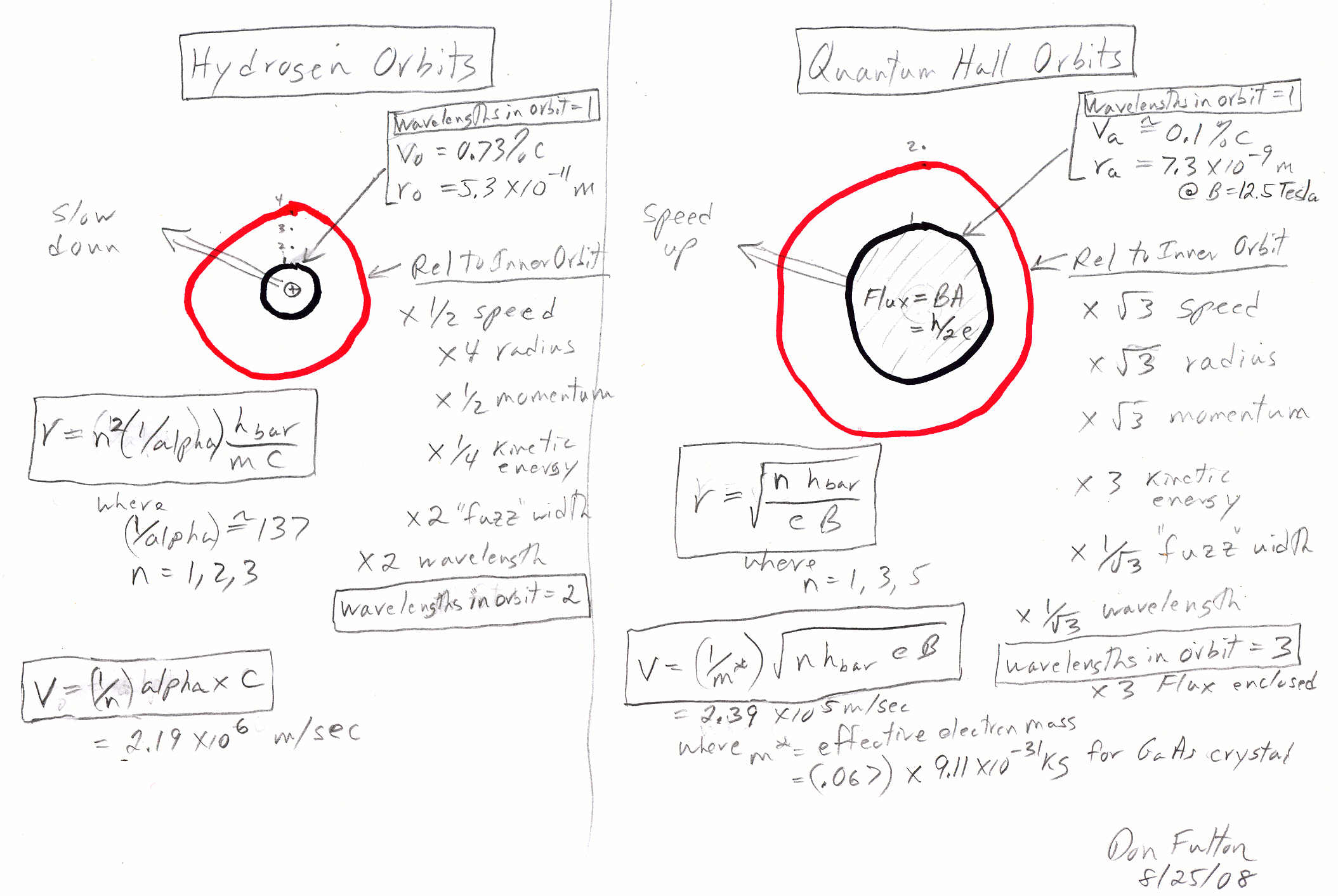
Quantum hall orbits & hydrogen orbits
Below I have
sketched out (side-by-side) the parameters of the two inner electron orbits
of hydrogen and a quantum hall device (@ 12.5 tesla and GaAs crystal).
The quantum nature of the inner orbits is similar, but the outer orbits
are different. One wavelength just fits in the inner orbit in both cases.
The inner radius of the quantum hall orbit is (approx) x137 larger than the (Bohr) hydrogen inner orbit, so based on (wavelength = h/p) the momentum of the hall electron must be (approx) x137 smaller than the hydrogen inner electron. The hall electron momentum is x137 lower due to x9.2 lower speed and an effective mass (in GaAs) lower by 1(/0.067) = 14.9.
In hydrogen outer electrons move relative to inner electrons slower, but in the quantum hall device outer electrons move faster. In hydrogen the velocity goes as 1/sqrt{radius}, whereas in quantum hall it goes as radius. Thus it is possible for electrons in inner and outer orbits in a quantum hall device to orbit in sync, which in fact they do! But how can outer electrons go faster, doesn't it take more force? Well, yes it does, but it's provided by the Lorentz force law [F = q(E + v cross B)]. As long as the outer electrons 'see' the same B as the inner electrons, they feel a quadrature (bending) force that rises linearly with speed (F =evB). In other words the B field, although quantized, is effectively uniform, so the larger outer orbits enclose more flux.
The red line below shows the 2nd orbit. In hydrogen with the electrostatic force falling off as 1/r^2 the radius of the 2nd orbit is four times the radius of the inner orbit. In this orbit the electron moves at half speed, doubling its wavelength, resulting in two wavelengths fitting into the orbit.
In a quantum hall device the 2nd orbit hold three wavelengths. The reason given, which I take on faith, is that two wavelengths are excluded by the Pauli exclusion principle. For the 2nd orbit to fit three wavelengths it needs to have a radius (& circumference) sqrt{3} larger with a sqrt{3} faster electron having a sqrt{3} smaller wavelength.
Effective width --- how can B vary and not change Rh
First,
the plateau is very flat, one experimenter measured it to be flat to (at
least) one part in 10^8, so in a quantum hall reference it is not required
to set B exactly in the center of the plateau. Why this was so I initially
found very hard to understand, finding the references and papers maddeningly
unclear. The problem was that classic hall was described in terms of equating
E with (vdrift x B), but when physicists described the flat plateau it
was in an entirely different language, all extended vs localized states
and filled landau levels, with nary a mention of vdrift!
After struggling with this for over a week, I finally realized the key to understanding the flat plateau is to think 'effective width' (width*). In a real quantum hall device the crystal is not perfect, there is random potential variation over the area of the device. Variations in B (or total charge density) cause regions of locally trapped electrons to expand or contract in area. Think how the the area of islands in a lake with a rough bottom would expand or contract as the level of the water in the lake rose and fell. The 'islands' of trapped electrons are trapped around peaks and valleys of the crystal random potential, so they are unable to drift and do not contribute to the current. Since the total area of the device is fixed, the (effective) conducting width of the hall device (extended states), is able to change as the localized (trapped electron) areas expand and contract.
The key classic hall equations are below, but I have replaced width with effective width (width*). The starting point is the force balance between qE and qvdrift B (Vh/width = vdrift B). In the equations below note that charge density (per unit area) comes from the equation for current, so the relevant (to quantum hall) charge density is the charage density only in the extended states, because only these states contribute to the current.
i = charge density (per unit area) vdrift width*
vdrift = i/charge density (per unit area) width*
Vh = vdrift B width*
= B width* i/charge density (per unit area) width*
= B i/charge density (per unit area)
In classic hall the width cancels, and it does in a real quantum hall device too. It doesn't matter that variations in B (or charge density) cause the effective width of the conducting part of the device to expand or shrink, width* cancels. Why? Assume for a minute that charge density (per unit area) in the conducting regions does not change (it does change if B changes). Then wider localized areas means an (average) conducting channel (width*) that is narrower, so vdrift must increase (inversely to width*) if current (i) is held constant. A higher vdrift means a higher electric field (E) is needed to balance a higher (vdrift x B) force, but (here is the key) E automatically rises when the channel narrows, without Vh changing, because E = Vh/width*. Vh depends on the product of (vdrift and width*), and this product is constant when vdrift varies inversely with width*.
In the equation for Rh both width* and vdrift drop resulting in Rh dependent only on the ratio of B to the charge density (per unit area), which has to be interpreted as the charge density that contributes to the current, in other words the (average) charge density of the extended (conducting) area of the device. While the total charge density of the device is nominally constant, the available charge can redistribute between localized (trapped) and extended (conducting) states as B varies. Bottom line
Rh = B/charge density (per unit conducting area)
In the conducting areas the physicists say the landau levels are full and this region is incompressible. What this means (in english) is that the this region is totally full of electrons in a uniform matrix of cyclotron orbits (one, two, etc electrons per orbit).
Because flux (BA) is quantized, cyclotron orbit area is inversely proportional to B. A 10% increase in B results in the area of a flux quantum shrinking by 10% (approx) causing the area of electron cyclotron orbits to tighten 10% (approx). Since all the minimum flux quantum cyclotron orbits are occupied in the conducting area are occupied, charge density (per unit conducting area) increases 10% when B increases 10%. This is (another) key.
charge density (per unit conducting area) = e/cyclotron orbit area
= e/(h/eB)
= Be^2/h
Rh = B/charge density (per unit conducting area)
= B/(Be^2/h)
= h/e^2
On a plateau, where the number of electrons in an orbit is constant, charge density goes up as B and since Rh depends only on the ratio of B to charge density, B drops out and Rh stays constant on the plateau as B varies! The change in Rh from plateau to plateau is caused by changing the number of electrons in each orbit, the ith plateau having i electrons. The ith plateau also has an area (at the center of the plateau) i times larger than the top plateau, so from plateau to plateau the change density is nominally constant. With the denominator in the Rh equation constant (from plateau to plateau) Rh plateau values can be seen to drop linearly as B. Small reductions in B (on a plateau) cause no change in Rh because charge-density increases (as B).
Larger reductions in B at some point cause the number of electrons in each orbit to bump up by one (the charges required coming from localized states). An increase in the electrons in orbit causes the value of Rh to drop down to the next plateau because the charge-density (at the center of the plateau) is restored. This integer increase in electrons in orbit (as the orbit expands with reduced B) explains why Rh has plateaus and why they occur as all submultiples of 25.8k.
The fully occupied cyclotron orbits in the conducting area of the device also explain why Rh does not change when total charge density in the device varies. Charge can vary across the device area. Changes in total charge density result in only in the # of electrons (& charge density) of the (localized) electron areas changing, and this has no effect on Rh.
Considering the crystal --- extended and localized
states
Extended states
carry all the current from one end to the other. Extended states, which
are only a small fraction of the electrons states in the device, are totally
filled (physists call this state incompressible) with electrons whirling
in cyclotron orbits and drifting slowly through the device to form the
external current. All the rest of the device has localized states, which
is are only partially filled with electrons. These electrons also whirl
in cyclotron orbits, but they do not drift or contribute to the current,
because they are bound locally by random energy peaks and valleys of the
crystal.
The saturated, extended states current can be visualized as a narrow twisting river flowing through the middle of the device with boulders (localized states) strewn in the channel. Later work has revealed that the current flow of of the extended states may be very complex involving tunneling and so-called percolation in it.
At first I though it was possible to say how the area of extended states, i.e. the width of the 'river', expanded or contracted when B or flux density on the plateau change. Looking at state density figures (see below) it appears that localized states (probably) fill more when charge density increases and deplete when B increases (because high B causes the density lobes to expand upward in energy). At the same time higher B means less area is required for each electron because cyclotron orbits shrink.
I no longer think there is any clear-cut (total) area change as charge density or B change (on the plateau). It just depends too strongly on the nature of the crystal, but (and here is the key) it doesn't matter. As the key quantum hall equations (below) show any variation in the width or flow (vdrift) of the extended states 'river' cancel out of the equation for hall resistance (Rh). The 'river' width is the effective width of the quantum hall device. If it narrows and current is held constant, then vdrift increases just enough such that hall voltage (Vh) is unchanged (if B is unchanged).
Key quantum hall equations
force balance
E = Vh/width = vdrift x B
vdrift = Vh/(B width)
current
i = charge-density width vdrift
vdrift = i/(charge-density width)
equate
Vh/(B width) = i/(charge-density width)
Rh = Vh/i = B/charge-density (in extended states)
The equations above show quantum hall voltage depends only on the ratio of B to charge density (in extended states). The reason the relevant charge density is the charge density of extended states is that the charge density comes from the equation for current and only the extended states contribute to the current.
We can now see why the quantum hall device works as a practical resistance standard, why modest variation in B or (total) charge density do not matter.
* Charge density variation
The energy lobes show that all quantum states in the extended regions ('river') are full. Meaning every flux quantum in the part of the device has exactly the same (one, two, etc) electrons whirling around it (depending on the plateau). It is full of charge, so any change in total charge density, which is a change in the total number of electrons in the device, must mean all the change takes place in localized regions. Hence the charge density appearing in the Rh equation is unchanged by changes in total charge density.* B variation
B appears in the numerator for the equation for Rh, so for Rh to be invariant to B [charge-density (in extended states)], which appears in the denominator, must increase linearly with B. It does. Above the argument is made that all the quantum fluxes in the extended 'river' are surrounded by electrons in cyclotron orbits. Since flux is (B x area), and quantum flux is determined by fundamental quantities (h/e), then the area of a flux quantum goes down inversely with B. This is confirmed by the radius of a cyclotron orbit that goes down as the square root of B (r = sqrt{n hbar/eB}. Whether extra electrons come from localized areas to keep the extended conducting 'river' approximately constant, or whether it gets smaller is a don't care conditions. Since on a plateau, where the number of electrons in each orbit is constant, the charge-density of electrons (in cyclotron orbits) in conducting extended states changes linearly with B. Rh being equal to [B/charge-density (in extended states)] is thus invariant to changes in B on a plateau.Orbits and plateaus
It's tempting to assume that since Rh plateau values exist at (nearly) all interger submultiple values (1/2, 1/3, 1/4 etc) of a reference value (25.8k) to assume the plateaus differ by some interger count. For example, maybe the plateaus differ in the number of electrons in orbit, or the number of flux quanta encircled, but can this be quantified?
Reference equation
I'll take
as my starting point what I think is the most fundamental integer hall
equation. It can be rewritten in terms of the electrons in orbit and orbit
area, because charge-density is just the number of electrons in an orbit
divided by the area of the orbit.
Rh = B/charge-density (in extended states)
= BA/(# of electron charges in orbit of area A)
= flux in area A/(# of electron charges in orbit of area A)
Highest plateau
Is there a
plateau at Klitzing's constant (25.8k)? Probably. The Rh vs B figures
in a lot of quantum hall references do not show it. It's not shown in von
Klitzing's Nobel lecture nor is it in the French metrology graphs, which
at 50+ graphs is the most comprehensive quantum hall data set I have seen.
It's not used by the metrology labs, which typically use i=2 (Rh=12.9k).
However, it does appear on David Leadley's quantum hall site (see above).
It's the plateau labeled pxy = 1.0 x h/e^2. It's hard to know how close
any of these plateau curves are to real data, because they all look cleaned
up and idealized to some extent, especially Leadley's and the French's.
Presumably, the topmost Rh plateau (if it exists) would be one electron in a cyclotron orbit encircling one flux quantum, which is either h/e or h/2e depending on definition and exactly how the radius of the orbit is defined.
Flux quantum
An interesting
feature of cyclotron electron orbits is that (at constant B) electron velocity
goes up linear with radius (& with sqrt{area}). Electron (kinetic)
energy goes as velocity squared, so we can say energy goes up as area.
Now one flux quantum is either h/e or h/2e, depending on definition. As
the figure below shows, the smallest energy quanta (some references
call this 'zero-point energy') is half the size of larger energy quanta
[(1/2) hbar w -vs- hbar w]. So it's reasonable to expect (semi-classically)
that at high energy, high B, on the 25.8k plateau that all quanta are larger.
Let's see what happens if we set the flux to be the smaller flux quanta (h/2e) and assume one electron in orbit:
Rh = flux in area A/(# of electron charges in orbit of area A)
= (h/2e)/e
= h/(2 e^2)
= 6.629 x 10^-34/2 (1.6 x 10^-19)^2
= 12.9k
At 12.9k we are on the 2nd plateau because we get only half of the von Klitzing constant of 25.8k. To get Rh = 25.8k we either need to double the numerator or half the denominator, but there is no such thing as a half an electron, so we can't reduce the denominator! Hence to get the top plateau (Rh=25.8k) we must double the numerator flux to (h/e), which is the larger of the flux quanta. (h/e is the flux quanta value von Klitzing's uses in his paper.) Thus at the top plateau (25.8k) the 'flux in area A' and '# of electron charges in orbit of area A' are both uniquely determined.
For i=2 (Rh = 12.9k) there are two combinations of flux quanta and electron count [Rh = flux in area A/(# of electrons in orbit of area A)] that work, either the flux (in the numerator) must be halved or the # of electrons in orbit (in the denominator) must be doubled.
Wavelength
In the equations
below I show that one wavelength for i=1 (Rh =25.8k) just fits around the
smallest flux quantum of (h/2e). Hence a double area orbit encircling (h/e)
flux (at the same B) has a sqrt{2} higher circumference and a sqrt{2} higher
orbital velocity, meaning a sqrt{2} smaller wavelength, so it holds two
wavelengths.
Check (@ Rh =25.8k experimentally B is about 16 tesla)
BA = h/e
A = h/eB
r = sqrt{h/(pi eB)}
v = eBr/m*
wavelength = h/m*v
= h/(m*eBr/m*)
= h/(eBr)
Finding (circumference/wavelength) ratio
2 pi r/wavelength = 2 pi r/(h/(eBr))
= (2pi eB)/h x r^2
= (2pi eB)/h x h/(pi eB)
= 2
checks --- two wavelengths fit around an (h/e) flux quantum on Rh=25.8k plateau.
Wavelength vs B
Quantum electron
cyclotron orbit quantization is entirely independent of B. As B decreases,
the radius of the cyclotron orbit increases and the electrons move slower
causing the wavelength (wavelength = h/m*v) of each electron
to increase just enough so the same integer number of wavelengths
still fit into the orbit at all B, . Both radius and wavelength
change as (1/sqrt{B}).
Plateau 1
Rh = 25.8k (Bref, Aref)
area flux = h/e
# of electrons in orbit = 1
wavelengths = 2
Plateau 2
Rh= 12.9k (Bref/2, 2Aref)
area flux = h/e
# of electrons in orbit = 2
wavelengths = 2
or Rh= 12.9k (Bref/2, Aref)
area flux = h/2e
# of electrons in orbit = 1
wavelengths = 1
Plateau 3,4,5 etc
So what combinations
work at lower Rh values?
First thought
I initially
thought the answer was simple. Just hold the number of electrons in orbit
at one (denominator = 1) and hold the area of the orbit fixed at
(Aref). Then as B (in the numerator) goes down flux in the (fixed) area
goes down resulting in Rh going down with B. B at 1/3rd, 1/4th, etc of
Bref results in Rh at 1/3rd, 1/4th , etc of 25.8k. Simple, but there is
a serious problem.
The problem is that at the 2nd plateau the flux in the orbit area is already at its minium quantum value (h/2e). If we take flux quantum as a hard limit, then we can't have electrons circulating around pieces of flux that are smaller than (h/2e). This approach doesn't work.
An approach that works
Looking at
the Rh equation(s) we can see there is another approach. As B goes down
let the area of the orbit expand (inversely with B). This hold the 'flux
in area A' (numerator) fixed at a flux quantum (h/e). To reduce Rh the
number of electrons on each plateau is increased by one, i.e. three electrons
on the 3rd plateau (Rh = 1/3 x 25.8k), four electrons on the 4th plateau
(Rh= 1/4 x 25.8k), etc. We can see from above that this pattern works too
for plateaus 1 and 2. So for the nth plateau we have
Plateau n
Rh= 25.8k/n (Bref/n, nAref)
area flux = h/e
# of electrons in orbit = n
wavelengths = 2
This approach has two additional huge advantages: one, it explains why plateaus exist, i.e. why small changes in B makes no changes in Rh, and two, it explains why plateaus occur at interger submultiples of von Klitzing's constant (25.8k).
** Plateau's are flat because small changes in B don't cause any flux change since as B goes down area goes up. In the equation [Rh = flux in area A/(# of electron charges in orbit of area A)] therefore both the numerator and denominator are constant. Using the formula [Rh= B/charge-density (in extended states)] the explanation is that as B goes down charge-density goes down too as a fixed number of electrons are spread over more area.
** The interger nature of the plateaus, of course, directly follows from the integer number of electrons in orbit around the flux quanta: one on plateau #1, two on plateau#2, etc. And since the number of electrons appears in the denominator of Rh, plateaus of Rh occur are at integer submultiples of the maximum value (25.8k).
The figure below shows how cyclotron orbit size varies with B. B ten times larger (right) has ten smaller cyclotron orbits in the same area of the one large orbit (left). Not shown in the figure is that the number of electrons in both (blue) cylinder areas is constant keeping the charge density constant. So if right represents the (i=1) top plateau, then it has one electron per orbit and Rh=25.8k, while the left orbit has ten electrons and Rh = 2.58k, since [Rh = B/charge-density (in extended states)].
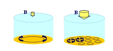
Cyclotron area vs B, right B = x10 left B(M. Fleischhauer,
Technische Univsitat Kaiserslautern)
Corollary
(Seems to
me) this approach must be right. It just explains too much. But if it is,
then there is a corollary --- it severly constrains the properties of cyclotron
orbits. Cyclotron orbits must be nothing like Bohr orbits. In a Bohr hydrogen
atom one or two electrons fit in the same inner orbit, and eletrons (3
to 8) are in orbit(s) with a radius four(?) times the radius of the inner
orbits.
In the (semi-classical) picture we have derived for cyclotron hall all electrons are whirling about a flux quantum (h/e) at the same radius (to encircle fixed flux). As B decreases and the orbit area expands with the number of electrons in the same orbit increases as 1,2,3,4,5 etc as plateaus decrease.
How to all these electrons fit into one orbit.? No reference I have found addresses this. There is no mention of (the equivalent) to quantum numbers that electrons have in Bohr orbits. One possibility that the theorists discuss (to explain fractional hall) is that electrons pair up forming quasi-particles that act like boson. This would kill the exclusion principle that applies only to fermions.
Confirmations
NTSB paper --- Cyclotron
radius = sqrt{hbar/eB} for orbits of the first landau level, in which case
each
electron
of the 2DEG has trapped a magnetic flux of quantum (e/h).
One reference states: " If the path encloses a single flux quantum (h/e) ... fermionic electrons can be formally converted to bosons"
NTSB paper --- "Cyclotron orbital velocities vectoriially tend to cancel everywhere within the device except near the device periphery" So with B, but with no external current, a current circulates around near the outside edge. (about 1 ua at B=0 and 0.8ua at B=12 tesla)
Experimental value of B
I thought
at one point I could derive some plateau information from the experimental
value of B. This didn't work out, still it's interesting to look at the
data. Clearly the values (@ Rh =25.8k) are all in the same ballpark but
are not really the same. The difference is probably too large to be B measurment
error, so it's likely due to crystal (or other sample) differences. Reading
from the graphs of the three figures in this essay B in the center of the
(extrapolated) 25.8k plateau is
von Klitzing
4 x 4 tesla
16 tesla
Leadley
2 x 7.5 tesla
15 tesla
French
3 x 6 tesla
18 tesla
Rh = B/charge-density (in extended states)
Rh = BA/(# of electron charges in orbit of area A)
= flux in area A/(# of electron charges in orbit of area A)
B = (Rh/A) (# of electron charges in orbit of area A)
Since Rh and # of electron are tightly defined, it would appear that small variations in B like 10% must be due to variations in cyclotron area (A), probably due to variations in crystal parameters.
Quantum hall physics details
Excellent
recent 2004 letter to Nature (Israel and Germany) on measurments of
electron transport profiles in quantum hall --- http://www.fkf.mpg.de/klitzing/publications/pdffiles/MPI-VK1037.pdf
--
Local orbits are in concentric circles. When B increases all orbits
shrink to maintain constant flux through their area. "Thus at higher B
there are
more states per unit area"
-- for a given B the (local) electron density cannot exceed nmax, which
is one electron
per flux quantum, so as electrons are added local regions form where n
reaches
nmax (all the landau states are full here). n=nmax regions are "incompressible"
and exist as island in compressible regions where n<nmax. A compressible
region
surrounded by an incompressible region behaves like a 'quantum dot'.
** Notice, this explains the straight lines. When B is doubled nmax doubles,
so the imcomressible region forms at n (charge density, set by
varying voltage on transistor gate) twice as high.
-- their
baseline is the incompressible line (labeled 1). Here the whole landau
region
is incompressible. When density (or B?) is changed compressible islands
appear
in the landau landscape. These compressible pockets surrounded by
incompressible (filled state) regions act like quantum 'anti-dots'
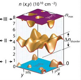
(my interpretation) Their picture is of island patterns (either compressible -non full states, or incompressible island --full states) created by water over an bumpy surface. B sets nmax, which is the level of the water. Ndisorder is a measure of the degree of bumpiness. Presumably as B changes (over a range) islands expand or contract, but their number (& location) stays (reasonably) constant.
 .
. 
Extended states, which are the only states that conduct the current, exist only at the 'core' of the Landau levels. Core landau states are full on the hall plateaus. The energy separation between Landau levels (except the lowerest) is (hbar w), which is the kinetic energy of the cyclotron electrons. It is observed that on the hall plateau the hall current tends to concentrate near the device edges while it diminishes on average in the device interior as a consequence of localization.
 .
. 
Calculated local spacial
density variations
Measured compressibility (at a point) plotted vs charge density (n) and
B.
Level III is nearly full Landau level (flat
is full) Slope of
'1' line is equal to fundamental units (n/B = e/h)
Left
The left figure
shows how even though total charge density is (normally) constant,
i.e. the total number of (non-crystal trapped) electrons is constant in
the device, the local charge density varies across the device. This variation
is due to electrons moving around to screen random local potential peaks
and valleys in real (dirty) crystals.
Saturation in local charge density (marked Nmax) is due to the quantum nature of electron cyclotron orbits. When one (or an integer number) electron is orbiting all the quantum fluxes in a region of the sample, local charge density can increase no more. Nmax is only constant if B is constant. Cyclotron orbit areas go down inversely with B, so Nmax increases linearly with B. Changes in the total charge density of the semiconductor affect how many orbits can fill, but do not change Nmax. The III level in the figure is a landau level that is almost, but not quite, full of electrons. The full areas are where it is flat and local charge density is equal to Nmax. These regions are referred to as "incompressible" and are the regions of the device that carry the current.
When the extended landau states are saturated (at Nmax), an increase in (total) charge density causes the additional electrons to go into localized states where they are trapped and do not contribute to the current. Rh is equal to the ratio of B/charge density (extended states), and since charge density (of extended states) doesn't change when total charge density changes (on the plateau), Rh is constant.
On the other hand an increase in B causes electrons to move from localized states to added extended states (at lower energy), thus keeping the extended state charge density saturated at a new higher Nmax. Higher Nmax with higher B is due to a reduced area of flux quanta and cyclotron orbits. Rh is equal to the ratio of B/charge density (extended states), and since charge density (of extended states) increases (& decreases) linearly with B, Rh is invarient (on the plateau) to changes in B.
Right
Measured data
in right (above) shows another way quantum hall is quantized with values
that depend only on fundamental quantities. By wiggling the gate voltage
(on a transistor) and using a tiny localized probe positioned above a random
point of the quantum hall device researchers were able to measure whether
the electron 'gas' at that spot was compressible or incompressible. Charge
density and B were then varied over a wide range and the compressibility
plotted vs (total) charge and B.
The bright regions on either sides of the (blue/purple) lines are quantum hall plateaus, so in effect the lines identify the B (for a given total charge density) at the center of the plateaus.
The result is a series of lines that when extrapolated go through the origin. The slope of the lines, in units of (charge density in electrons per m^2) over (B in tesla), come out to be integer (or factions) of (e/h). Neat! Reading off the figure (for the line marked '1') I get the following:
n/B (read off graph) = e/h
11.5 x 10^14 m^-2/4.8 tesla = 1.6 x 10^-19/6.6x 10^-34
2.4 x 10^14 = 2.4 x 10^14
confirmed
------------------------------------------------------
Key experimental data (9/1/08)
In trying
to figure out the various quantum hall orbits the data from the Weizmann
Institute (above, right) looks very interesting. It purports to be real
data published in the journal Nature (though how massaged it is is hard
to say). The numbers 1,2,3,4 along the top clearly indicate the plateaus,
and the axes give values for charge density and magnetic B field. (One
thing that's a little strange about the Weizmann data is how low the B
values are, though this can be explained if they are using a material with
a very high charge density.)
Eyeballing this plot I read that at B = 4 tesla the charge density on the 1st plateau (Rh = 25.8k) is 9.6 x 10^14 charges/m^2 (approx) [Note the graph axis in cm^2. I have converted to m^2]. Reading horizontally we find the 2nd plateau (Rh = 12.8k) at B = 2 tesla and the 4th plateau (Rh = 6.4k) at B = 1 tesla. This pretty much 'proves' that the charge-density holds constant with Rh declining as B (on the various plateaus) consistent with the semi-classical equation Rh = B/charge-density (in extended states).
Let's see if the numbers work. Here's the top plateau, where we know Rh should equal 25.8k. (I will initially assume that they are counting electrons (not electron pairs)).
Rh = B/charge-density (in extended states)
= 4 tesla/(9.6 x 10^14 charges/m^2 x 1.60 x 10^-19 coulomb)
= 26.0 x 10^3
= 26.0k
checks (25.8k within < 1%)
Let's also check the French Metrology Lab data (from graph far above). The graph shows the 2nd plateau (Rh =12.9k) centered at 9.0 tesla and the 3rd plateau (Rh = 8.6k) at 6 tesla, so with high confidence we can extrapolate that the 1st plateau is at 18 tesla. Two slightly different charge counts are given 4.1 and 4.2 x 10^15/m^2, so let's use the average (4.15 x 10^15/m^2).
Rh = B/charge-density (in extended states)
= 18 tesla/(4.15 x 10^15 charges/m^2 x 1.60 x 10^-19 coulomb)
= 27.1 x 10^3
= 27.1k
checks (25.8k within 5%)
Conclusions
Data from
two labs appears to confirm the (derived) equation: Rh = B/charge-density
(in extended states). Both labs appear to count single electrons (not electron
pairs) per unit area. Rh declines (on the various plateaus) as B declines
with the charge-density holding constant.
------------------------------------------------------
Density of states
The gap in
the density of states that gives rise to the quantum hall plateau is the
gap between
extended states. The right figure (below) shows the
extended states are at the peaks of density lobes. In the left figure a
plateau exists in variations in B from level (a) and (b). As B increases
(a) => (b) the energy in the available states (cyclotron energy) rises,
but this energy is below Fermi energy so all the states stay full.
 .
. 
Quantum hall state
density vs B -- states fill to Firmi level (Ef)
State density profile -- Only extended states conduct current
(from David R Leadley quantum hall site)
Laughlin explained that the 'broading' needed to make a plateau requires a dirty system, meaning random potentials and to peaks and valleys in energy randomly distributed across the sample (marked delta 'n disorder' in figure above). The vast bulk of electrons are trapped in these 'localized' peaks and valleys, which do not move, thefore these electrons do not contribute to the current. The hall plateau is really flat.Experimentally it's flat to better than ±5 x 10^-8 over a 0.4 tesla range.
Only an extended state at high B is (exactly) in the middle of a an energy peak (Landau level). In high B not quite all the states are localized. Papers argue this system is very complex with incompressible strips in the sample running down the middle and localizing electrons. electrons are traversing the incompressible islands by tunneling. But only (mostly?) the center carries current.
Working through some quantum hall numbers
One way to
get some understanding of a new theory is to put in some numbers, so that's
what I did with the semi-classical quantum hall eqations. (When I did this
I was using (h/2e) as the flux quantum, which is the Wikipedia value, but
later analysis has convinced me that cyclotron orbits in a quantum flux
device encircle (h/e) flux on all plateaus.) Assume device is 5 x 10 mm
and B=10 tesla.
I will also assume GaAs which changes (in all equations I think) the electron mass (m) to the 'effective' mass (m*). m*= 0.067 m = 0.067 x 9.11 x 10^-31 kg = 0.61 x 10^-31kg.
flux = BA = 10 tesla x (10 mm x 5 mm)
= 5 x 10^-4 webers/m^2
Q = flux/Rh = 5 x 10^-4/2.58 x 10^4
= 1.94 x 10^-8 coulomb
# of electrons = Q/e = 1.94 x 10^-8/1.6 x 10^-19
= 1.2 x 10^11
Below I show that the number of electrons is equal to
number of flux quantums for i=2. Hence Q can be found from # of flux quantums
in device, and then Rh can be derived (Rh = flux/Q).
Rh (i=2) = h/2e^2 (see equations above)
1.29 x 10^4 =?= 6.63 x 10^-34/ 2 x (1.6 x 10^-19)^2
= 1.29 x 10^4 yup, checks
dQ/dt =idrift = 50 ua
= 5 x 10^-5 coulomb/sec
electron 2D density = 1.2 x 10^11/50 x 10^-6 m^2
= 2.4 x 10^15 electrons/m^2
so
time for electron to travel 10 mm
= Q/(dQ/dt) = 1.94 x 10^-8/5 x 10^-5
= 0.39 x 10^-3 sec
electron drift vel = 10^-2 m/0.39 x 10^-3 sec
= 25.6 m/sec
electron DeBroglie wavelength @ drift vel = h/p = h/*mv
= 6.63 x 10^-34/(0.61 x 10^-31 x 25.6)
= 0.42 x 10^-3
check (flow of charge in one sec)
dQ = (electron 2D density) x drift vel x width
= (2.4 x 10^15 electrons/m^2) x (25.6 m/ 1 sec) x 5 x 10^-3 m
= 3.07 x 10^14 electrons x 1.6
= 3.07 x 10^14 electrons x 1.6 x 10^-19 coulomb/electron
= 4.9 x 10^-5 coulomb checks
Flux quantum (Wikipedia) is h/2e (inverse of Josephson constant). The flux quantum is (almost) measurable in superconducting systems using a SQUID, the most accurate magnetometer known.
flux quantum = h/2e = 6.626 x 10^-34/ 2 x 1.6 x 10^-19
= 2.068 x 10^-15 webers/m^2
# of (h/2e) flux quantums in Hall device
= flux/flux quantum = 5 x 10^-4/2.068 x 10^-15
= 2.42 x 10^11 (exactly twice
the nunber of electrons!)
Note, the area of an (h/e) flux quantum (at the same B)
must be twice an (h/2e) flux quantum, so
# of (h/e) flux quantums in Hall device
= 1.21 x 10^11 (exactly same as
the nunber of electrons!)
Neat --- One ref says electrons natural pair up with
two
flux quanutum form composite fermions that also orbit. If Rh=12.9k (i=2),
then number of electrons equals number of (h/2e) flux quantum.
area per quantum = flux/B = 2.068 x 10^-15/10
= 2.068 x 10^-16 m^2
check
area per quantum flux = 5 x 10^-5 m^2/2.42 x 10^11
= 2.07 x 10^-16 m^2
sq lin dim of quantum flux = sqrt{2.07 x 10^-16 m^2}
= 1.43 x 10^-8 m
Cyclotron frequency
is the frequency of electrons circling magnetic field lines. It is apparently
related to a quantization in angular momentum, which is hbar x w (angular
freq). m in the eqattion below may be 'corrected' mass. (Yup, correct mass
is smaller by factor of 15, so wc is correspondingly higher 2.65 x 10^13
rad/sec on one ref)
w (angular freq) = eB/m*
= 1.6 x 10^-19 x 10 tesla/0.61 x 10^-31
= 2.62 x 10^13 rad/sec (independent of radius) (agrees
with French ref)
equate the circular cyclotron orbit area to square quantum
flux area
(sq lin dim)^2 = pi r^2
r = sqrt{1/pi} sq lin dim
= 0.564 x 1.43 x 10^-8 m
= 8.1 x 10^-9 m
(agrees with French ref)
cyclotron vel of electron is orbit length (2 pi r) divided
by (2 pi x time to move a radian) = r/(1/w) = rw
v = rw
= 8.1 x 10^-9 m x 2.62 x 10^13 rad/sec
= 2.12 x 10^5 m/sec
(slow < 0.1% speed of light)
kinetic energy
E = (1/2)m* v^2
= (1/2) 0.61 x 10^-31 x (2.12 x 10^5 m/sec)^2
= 1.37 x 10^-21 joule
cyclotron (or gyroradius) radius (wikipedia)
r = m*v/eB = velocity/cyclotron radial freq
= 2.12 x 10^5/2.62 x 10^13
= 8.1 x 10^-9 m (Yup, 1.13 = sqrt{4/pi}
larger than half of
sq lin dimension and pretty close (ignoring x 1.13)
it's 7.2 x 19^-9 to the Bohr radius/alpha
(7.4 x 10^-9m)
check
r = sqrt{n hbar/eB}
= sqrt{1.05 x 10^-34/1.6 x 10^-19 x10}
= 8.1 x 10^-9 m OK
circumference =
2 pi x 8.1 x 10^-9 m
= 5.09 x 10^-8 m
orbit time = circumference/angular speed
= 5.09 x 10^-8 m/2.12 x 10^5 m/sec
= 2.40 x 10^-13 sec
orbit freq = 1/2.40 x 10^-13 sec = 4.16 x 10^12 hz
hence effective loop current (i =dQ/dt) is charge
e per rotation time?
i = 1.6 x 10^-19 coulomb/2.40 x 10^-13 sec
= 0.67 x 10^-6 A (0.61 ua)
presumably this would be the same current as rotating outside
(close to NIST value of 0.81 ua @ B=0)
time for electrons to orbit (at cylotron speed) around
edge of device
edge time = distance/cyclotron velocity
= 2 (10 +5) x 10^-3 m/2.12 x 10^5 m/sec
= 1.42 x 10^-7 sec
However, it can be argued that the electrons at the edge
appear to move just two radii every orbit time. This is pi less distance
than the circumference, so 'edge velocity' would be pi less than cylotron
velocity. Hence from this point of view
edge time = distance/'edge velocity'
= distance/(1/pi) cyclotron velocity
= pi distance/cyclotron velocity
= pi 1.42 x 10^-7 sec
= 4.46 x 10^-7 sec
deBroglie wavelength = h/p = h/m* x v
wavelength = 6.6 x 10^-34/0.61 x 10^-31 x 2.12 x 10^5
= 5.10 x 10^-8 m
Yes!! one electron De Broglie wavelength (at slow rotation speed) just fits (5.10 vs 5.09 x 10^-8) into the cyclotron orbit (at i=1, 25.8 kohm). A wavelength of 51 nm also meets the requirements mentioned by von Klitzing that for a 2D electron gas the vertical potential well (typ 10 nm) must be small compared to the deBroglie wavelength. (If you double radius (at same B), then since orbit time stays the same, the electron must go twice as fast, so its wavelength is half, therefore four wavelengths would fit in this double size radius.)
It's tempting to consider the current is many whirls around flux lines distributed evenly across the sample. But this is a superconducing sample, and NIST paper shows the current mostly (not all) circulates around near the outside edges of the sample.
How is the hall voltage measured?
I initially
didn't see how the hall resistance could be measured so accurately, to
something like one part in 10^9 to 10^10. You can't put a hall device in
classic resistance bridge because it is not a two terminal device. The
voltage is measured on one set of terminals and current on another set
of terminals, and the values are small only 645mv @ 50ua for i=2.
It turns out that in the superconducting world there are some tricks that can be played which make ratioing circuits much more flexible. A key component is a cryogenic current comparator (CCC). This is essentially a DC transformer that allows isolated DC currents to be ratioed to something like a part in 10^9. With the proper the geometry the net flux of different number of turns of coils can be nulled by servoing current sources. The nulling device is a SQUID, which though I haven't studied it, I think is a quantum device that works down to a tiny fraction of one flux quantum. Below is a link to the a commercial quantum hall resistance standard plus CCC bridge (QHR2000) made by Cyrogenic Ltd of UK.
http://www.cryogenic.co.uk/downloads/brochures/qhr2000.pdf
Another technique is switching the input to the nulling voltmeter with relay contacts between hall terminals and a voltage across a reference resistor.
Quantum hall resistance standard history
In 1980 von
Klitzing is surprised to find that hall resistance at (very) high magnetic
fields and low temperatures is quantized. The plateau hall resistances
are immediately very interesting because they are found to be very close
(within 1/10th ohm) to the ratio of two fundamental quantities (h/e^2 =
25,812.807 ohm) and its integer submultiples. Von Klitzing has a simplistic
theory to explain Rh, but cannot explain why the plateaus are wide and
robust, which they are. In 1985 he wins the Nobel prize for physics for
this discovery.
In 1982 Laughlin, who will later explain the fractional quantum hall effect and for that win the 1998 Nobel prize for physics, reads von Klitzing paper and in a few days comes up with a deep argument, based on gauge invariance (whatever that is!), as to what is going on and why Rh should be equal to h/e^2. Laughlin talks about this paper in his autobiography, "The upshot of this theory was that (magnetic field) localization caused the effect (quantum hall) and that the Hall conductance was accurately quantized because it was a measurement of the charge of the object being localized, in this case the electron."
Many other groups around the world build and test quantum hall devices nearly everyone measures the same value (within 7 to 8 digits) for the hall resistance. The resistance is found to be very robust. It is invarient to the effective (electron) mass (hence to the type of crystal), to the disorder in the sample, and the dimensions of the sample. In 1990 the quantum hall becomes approved internationally as the new resistance standard, two orders of magnitude better than the old standard.
Amazingly it is not until 1988, eight years after the quantum hall effect is found, before anyone publishes a complete circuit model for it. Ricketts and Kemeny's model includes the effect of current flow in the hall sense terminals and models the voltage drop on the longitudinal (current) path. With a good circuit model in hand the effect of various error sources, like contact resistance and wire resistances, can be calculated.
Five years later (1993) Delahaye shows how to configure the quantum hall as an accurate two terminal device. Rather than using the side sense terminals (open circuit) to measure the hall voltage, he suggests some non-obvious (tricky) crossconnecting of the sense terminals and current terminals. Analysis of these new connections using the circuit model, confirmed by testing, showed that a feedback effect occurs that cancels out much of the effect of various stray resistances, like contact and wire resistance. This configuration also has potential to improve the performance of the quantum hall device when it is excited by AC.
Quantum hall circuit model
The quantum
hall circuit model (below) is very interesting. How it was derived I could
not trace since I was unable to access the Ricketts and Kemeny paper and
no one else seems to discuss it. It generates not only (classic) hall voltage
on the 3,4 sense terminals in proportion to current in the DS current path,
but also generates a hall voltage in the DS path if current flows in either
of the 3,4 sense terminals. Normally, of course, in classic hall operation
there is no current in 3,4 terminals since hall voltage is sensed with
a very high impedance meter.
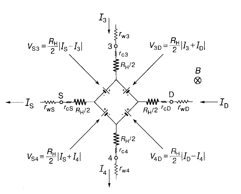
NIST quantum hall circuit model (one pair of sense
terminals)
The hall voltages are generated by four current controlled voltage sources with the equations shown in the figure. When there is no current in the 3,4 sense terminals, all four of the voltage sources are the same. This causes the voltage sources to cancel in the DS path, so the impedance in the DS path is just two Rh/2 resistors in series. In the 3,4 path the top/bottom voltage sources add creating the (classic) hall voltage.
Current path impedance puzzle
The really
puzzling thing about quantum hall circuit model is that it has resistance
in the DS terminals, in fact the same resistance (Rh/2) is in series
with every terminal. Rh, of course, is the classic hall resistance defined
as the open circuit sense voltage divide by the current in the current
path, so resistances in the model are typically of little interest . Rh/2
is a high value resistor typically equal to 1/4th of the von Klitzing (constant)
impedance (Rh/2 = 25.8k/4 = 6.45k typ) and consequently very stable.
Physicists claim current path has (nearly) zero resistance!
But doesn't
this conflict with the physics analysis that always shows the longitudinal
(DS path) resistance to be exactly zero on the plateaus? For a while
this drove me nuts. Even now it totally dumbfounds me that the voltage
across the current terminals is (virtually) never mentioned. How can everyone
say the longitudinal resistance is zero and not comment on why there are
these two large resistors in the current path of the circuit model? It
was clear to me from test data that the circuit model had to be right.
I must have read half a dozen lectures and textbook descriptions of the quantum hall effect and not one of them mentioned that in a quantum hall device there is a voltage across the current terminals that basically is the same as the hall voltage on the sense terminals. Every experimentalist must know this, but do the professors? Who knows, maybe not. Their simple theory shows the longitudinal impedance as zero, end of story?I eventually figured out that resistance between sense terminals on the same side (shown as RL in the device sketch below) is zero, so longitudinally, internally there is no resistance. The mystery resistors in the model arise (I am pretty sure) from crossing potential lines that ring the device near the edge. These potential lines come from currents that circulate around the device near the edges. This explains why all the resistors are the same; from any terminal you cross the same number of potential lines to get to the potential free interior. This potential lines are (sort of) a quantum potential described in terms of landau levels rather than an ohmic voltage.
Two terminal quantum hall resistance
Thirteen years
after it has has been invented, and three years after it had become the
international resistance standard, someone (Delahaye) figures out that
the quantum hall can be configured into a high quality two terminal device.
Delahaye shorts the sense terminals to the current terminals (they are
nominally at the same voltage) with the surprising result that errors due
to wire resistance in the current path are nearly eliminated!
Being a circuit guy I couldn't resist digging into Delahaye tricky crossconnected quantum hall circuit to see how it really works. Below I sketched out Ricketts and Kemeny's model with Delahaye's crossconnection of the sense terminals to the current terminals that makes the quantum hall into a two terminal device. Balanced mode is pencil and red shows values when a 2% unbalance resistor (100 ohm) is added to the drain terminal. To keep the numbers simple I set (Rh=10k) rather than its actual value for i=2 of (12.9k = 25.8k/2).
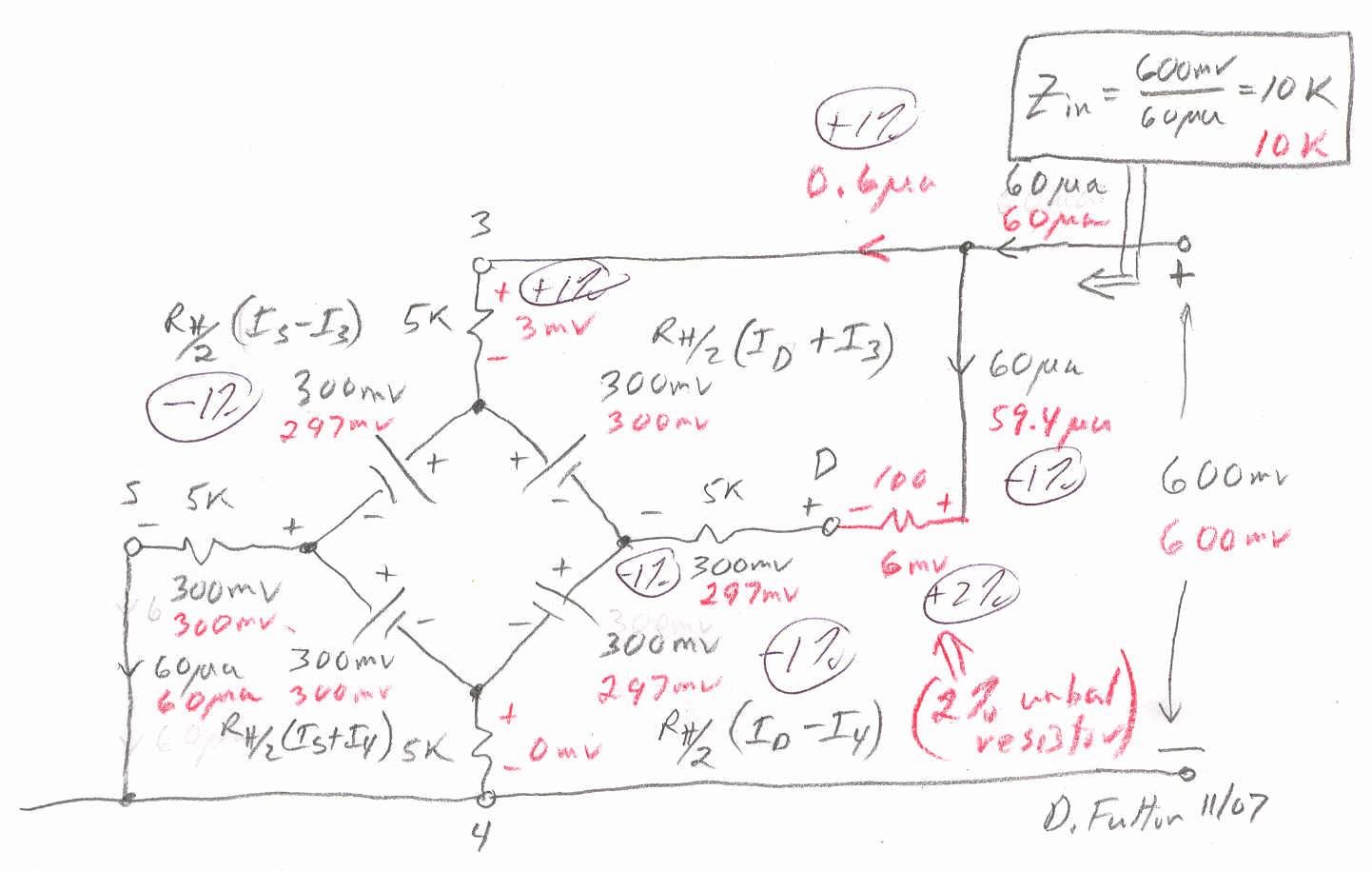
Two terminal quantum hall resistance circuit model
w/wo 100 ohm unbalance
(Rh here is rounded to 10k only to keep analysis simple.
Typical Rh=12.9k)
In normal operation (pencil) all the current flows in the horizontal DS path and no current flows in the sense terminals. This is because the open circuit sense terminal hall voltage, which is set by the four current controlled voltage sources, is always exactly (ideally) the same as the longitudinal Drain-Source voltage, hence there is no voltage across the sense Rh/2 input resistors when the terminals are connected.
Red shows new values when a 100 ohm unbalance resistor, simulating wiring resistance, etc, is added in series with the D terminal. Since it has about 60 ua through it, it introduces a 6 mv differential between terminals D and 3. What happens is that about 1% of the input current (600 na) diverts from the current path to the sense path, and this sense current causes a small hall voltage to appear in the current path.
* In the current path half of the 6mv across the 100 ohm voltage is compensated for by a small (rt/left) hall voltage induced by the small current (600 na) in the sense terminal, and the other half by a reduction in the voltage across the drain series Rh/2.
* In the sense path a 3 mv reduction in the (top/bot) hall due to 600 na less current in the current path is compensated for by a 3 mv increase in sense voltage due to 600 na flowing into the sense series Rh/2.The surprising result is that adding the 100 ohm resistor into the current path has caused neither the total input current (60 ua) nor input voltage (600 mv) to change. The two terminal input impedance is totally unchanged. Neat! A more exact analysis that takes into account 2nd order terms shows an impedance change of about a part in a million. But virtually all of that error is eliminated by Delahaye's triple connection that connects two sense terminals on each side to the current terminal. Test by NIST of the double and triple crossconnect circuits show the measured currents agree almost exactly with the model predictions, so Ricketts and Kemeny (non-obvious) quantum hall model is obviously very good.
References
NIST papers
with quantum hall circuit models
1) Crosscoupled current and sense configuration
http://nvl.nist.gov/pub/nistpubs/jres/100/6/j16jef.pdf
2) Cable effects
http://nvl.nist.gov/pub/nistpubs/jres/103/6/j36cag2.pdf
John Hopkins
quantun hall explanation
http://www.pha.jhu.edu/~qiuym/qhe/node4.html
Below is an
excellent set of 55 slides on quantum hall effect and metrology by French
standards lab:
http://www.metas.ch/LesHouches/downloads/talks/23_Poirier.pdf
Quasi-oddball
(but published) non-Schroedinger paper on quantum hall.
http://www22.pair.com/csdc/pdf/fqhpost.pdf
----------------------------------------------------------------------------
textbook Electron Materials and Devices by Ferry and
Bird
"(It) must be an odd integer so the wave function is antisymmetric."
"Quantization of electron cyclotron orbits arises from requiing that an
odd number of wavelengths fit into the orbit circumference."
-- Pauli exclusion requires an odd number of wavelengths fit into
cyclotron orbits
-- math is
simple
2 pi r = (2n +1) wavelength = (2n +1) (h/mv)
= 2 pi hbar/[(2n+1)mv ??
rearranged it gives
mv^2 = (2n+1)hbar w
E = (1/2) m v^2 = (2n+1)hbar w
r = v/w = sqrt{(2n+1)hbar/mw}
= sqrt{(2n+1)hbar/eB}